Introduction to vector databases – pgvector by example

All data can be vectorized – words, phrases, images, audio and documents. Vector databases are a tool which for most of the cases implements some kind of algorithm for approximating nearest neighbor which happens to be useful for similarity search between images or sounds and text, multiple contexts searching engines and LLMs improving domain-specific responses of large language models. When user provides the prompt, the feature vector is extracted, and the database is queried to retrieve the most relevant documents which then are added to the context of LLM and it creates a response to the prompt in this context. One of the most popular recently of the approximating nearest neighbor algorithms are Hierarchical Navigable Small World (HNSW) graphs which is one of the best performers in the benchmarks.

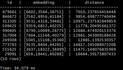
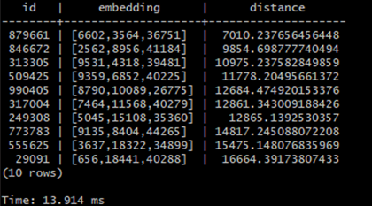
In this article I’ll try to familiarize you with this concept based on a simple example created using PostgreSQL plugin pgvector which introduces tools for storing, indexing and querying vectors inside postgres database and I will also show you how the indexing impacts the time of queries for the vectors.

For the installation of the environment, I’ll use docker as it’s the most effective and clean way. First, we should pull the docker image provided by pgvector creators to build our database.

docker pull ankane/pgvector

Next, we create the container with database using the pulled image.

docker run –name pgvector -p 5432:5432 -e POSTGRES_PASSWORD=secret -d ankane/pgvector

Then, we enter the container using bash (for windows users using git bash or cygwin there could be some issue related to TTY so prefix the command below with winpty).

docker exec -it pgvector bash

Connect to the database inside.

psql -U postgres -d template1

When we’re connected, we should provide the database with pgvector extension which comes with the pulled image.

CREATE EXTENSION vector;

For this example, I’ll create a simple table with columns representing id and three-dimensional vectors – those can be replaced by any size of vectors if you need, dependent on the AI model used to process the stored data and it’s output,

CREATE TABLE embeddings (id bigserial PRIMARY KEY, embedding vector(3));

Next, we can insert some data to populate the table for the testing purposes. For this we will create a simple sql script in our container using python script to generate random values for the vector embeddings. First we exit psql and then we create and save a file generate_random_vector.py with contents:

Pgvector plugin provides us with four distance functions to compare similarity of vectors.

• <-> – Euclidean distance
• <#> – (negative) inner product
• <=> – cosine distance
• <+> – L1 distance

In this example we will focus on the most popular which is Euclidean distance. The Euclidean distance between two points in Euclidean space is the length of the line segment between them. It can be calculated from the Cartesian coordinates of the points using the Pythagorean theorem. In general, for two points given by Cartesian coordinates in n-dimensional space the distance is equal to

This equation is important in the context of the AI as it’s an objective score by which we can summarize the relative difference between two vectors.

In this example we will try to query 10 most similar vectors to the one chosen by us and quantify the time spent on the query before and after indexing the table using HNSW algorithm.

For the query we will use distance operator provided by pgvector to calculate the distance between input vector and the stored vectors and then order them by the same distance. The example vector will be [434,3253,3343]. First, we need to connect to the database as before and then we can use a select query:

SELECT id, embedding, embedding <-> ‘[434,3253,33434]’ as distance from embeddings ORDER BY distance LIMIT 10;

The results can vary because of the randomness of stored vectors, but in my example the results are as follows

The time it took to process the query on a million vectors is equal to 94ms which is a pretty good feat. But let’s try to speed it up using HNWS indexing. The HNSW graph method offers an approximate k-nearest neighbor search which scales logarithmically even in high-dimensional data. An HNSW index in postgres creates a multilayer graph connecting stored data. It has better query performance than other indexing algorithm called IVFFlat but as a trade-off it has slower build times and uses more memory. The other advantage is that the HNSW index can be created without any data present in the table as IVFFlat requires a training step for it to work which means that data must already be present in the table for it to create an index. If we want to use Euclidean distance operator to query our table, we should use such a command

CREATE INDEX on embeddings USING hnsw (embedding vector_l2_ops);

The vector_l2_ops specifies which distance function we will use to query our table in this example it’s Euclidean distance, for inner product we have vector_ip_ops, for cosine distance it’s vector_cosine_ops and for L1 distance it’s vector_l1_ops. The HNSW can also be modified by parameters such as the max number of connections per layer, size of dynamic candidate list, also it has options for specifying querying and indexing built time. More information can be found in pgvector documentation. In my example creating an index on this table took 17 minutes and 21 seconds caused by the graph no longer fitting into maintenance_work_mem, which seems like a costly operation. But in exchange we get a faster response time on single queries.

The same query as before now takes significantly less time.

Indexing of vector embeddings using HNSW graph algorithm, provides a significant reduction in query time for the most similar vectors to our input vector. In this example the reduction was around 85% which can vary between the sizes of the table, dimensions of vector embeddings, platform memory and other factors.  This can be useful in real life applications such as chatbots or search platforms to provide the users with real-time answers to their queries. The main disadvantage of this approach is the time and memory required to index the database using the HNSW, if we swallow this inconvenience the pgvector plugin provides us with a great query tool with quick response times and easy usage to build the best AI based solutions and products.